Viz World User Guide
Version 17.0 | Published January 24, 2018 ©
GeoChart
![]()
The plugin can be found in the folder: Viz Artist 3: Built Ins -> Geom Plugins -> Maps-Adv.
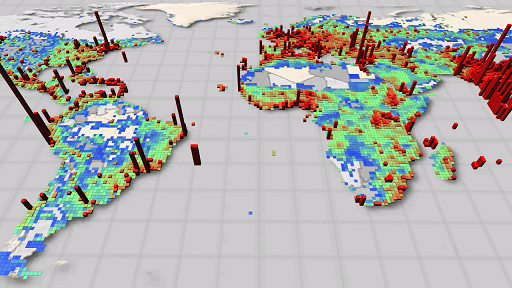
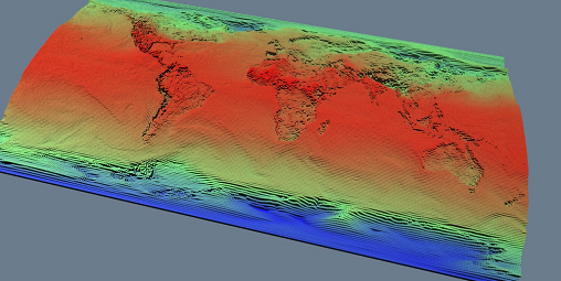
The GeoChart plugin shows geo-located values by representing them as 3D bars on a map. The data format can be a grid of geo positions (locations with constant distances from one another) or a list of coordinates. In addition, data may be split by timeframes and the plugin is able to animate the data chart throughout the frames.
In order to use GeoChart, it should be put beneath the geo reference and load data (see Supported Formats ). GeoChart will add the GeoChartShader to the container automatically.
This section contains information on the following topics:
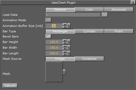
General
-
Load Data: Used to select the data file to be loaded.
-
Frame Number: When data comes in frames (see Supported Formats) this control appears and the desired timeframe can be chosen.
Please note that although it is possible to animate data through the Frame Number parameter it is not recommended because when the frame is switched the data is read from the hard disk such that such an animation will be more performance consuming. Moreover there will be no interpolation between frames such that the animation will ’jump’ from timeframe to timeframe. Use Animation Timeline instead. -
Animation Mode: Can be enabled if the data has timeframes. In this mode the whole frame sequence is analyzed and an animation is built. The data will be interpolated smoothly between the frames such that the animation will look smooth.
-
Animation Timeline: When an animation is built, the data can be animated through timeframes using this parameter.
-
Animation Buffer Size: Defines the size of the memory buffer in which the created animation is stored. If the buffer size is less than that required to build the animation from all the available frames, then not all of the frames will be included (You can check the total available frames by dragging the Frame Number parameter to the right and seeing the largest frame shown, and the frames included in the animation by dragging the Animation Timeline parameters to the far right).
-
Bar Type: Defines the geometry of the bar. Please note that Cylinder geometry is the most performance consuming while Prism is the lightest.
-
Bevel Bars: Bevels bars edges.
-
Bar Height: Scales the height of the bars
-
Bar Width: Scales the width of the bars
-
Bar Length: Alters bar’s length starting from the bottom.
-
Mask Source: Data may be clipped to a specific region such that only bars inside the region will be seen. For this purpose a mask image is required. You can drag the image into the ’Mask’ rectangle in the ’Image’ option or specify a container with a mask image in the ’Container’ option. See Creating Mask Images.
-
Rebuild : Only three parameters of the GeoChart plugin can be changed ’on the fly’ - Bar Height, Bar Width and Bar Length. Altering other parameters will require a Rebuild.
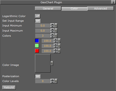
Color
-
Logarithmic Color: This option applies logarithmic scale to a color transform. This may be used when the data has dramatic differences between low and high values (in such cases the high values will be red by default and all the low values will be blue). Logarithmic scale makes this difference less dramatic, such that more in-between colors will appear on lower values.
An example of such data may be world population density. In large cities this value will be considerably higher than in it’s surroundings, making it difficult to see less dramatic differences in low population areas. -
Set Input Range: Constrains input range to a specified Input Minimum and Input Maximum value. All values below the minimum will be interpreted as lowest possible bar height (zero by default) and all values higher than the maximum will be interpreted as a maximum bar height. Note that when ’Set Input Range’ is pressed the actual minimum and maximum data values from the loaded data are seen.
-
Colors: The color map is defined by choosing colors and a number of in-between color ramp stages.
-
Color Image: Alternatively to using ‘Colors’, you can use an image to define the color map. The image must be dragged to this control. An example of an image defining color map:

-
Posterization: Enables a continuous color map to be split into a desired number of discreet colors.
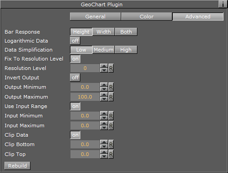
Advanced
-
Bar Response: Defines which property of the bar will be effected by the value it represents.
-
Logarithmic Data: Puts the values that the bars represent on the logarithmic scale. This gives a better indication of differences between low values, and makes the difference between low and high values less dramatic. May be useful in cases where there is a large difference between low and high values. (e.g. world population density). Consider using this option in combination with the ’Logarithmic Color’ option under the Color tab.
-
Data Simplification: The data file that is being loaded to a plugin may contain a huge amount of data and can become very performance intensive during rendering. For that reason you may want to resample the data and create different resolution levels to show lower resolution from farther distance. Moreover, data is spit into tiles by a culling mechanism. This parameter defines how may resolution levels will be created out of the original data, and therefore effects loading time and the animation built process.
-
Fix To Resolution Level: In some cases you would not like the data to be resampled, since this means a loss of some information. In such a case you can choose the option to use only one, fixed resolution level, which you choose by using the Resolution Level parameter. A zero value means that raw data is used. Raw data is not resampled and not split to tiles.
-
Invert Output: Maximum values get the lowest bar heights and vice versa.
-
Output Minimum: Defines the height of the bar representing the minimum found value.
-
Output Maximum: Defines the height of the bar representing the maximum found value.
-
Use Input Range: Defines the input range such that values lower than Input Minimum will be considered as having the Input Minimum value, and values higher than Input Maximum will be considered as having the Input Maximum value. This may be useful when focusing on a specific range in values.
-
Clip Data: Enables clipping the bars representing values lower or higher than defined in the Clip Bottom and Clip Top parameters. Note that when this button is switched to ’On’ the Clip Bottom and Clip Top controls appear with values corresponding to the actual minimum and maximum found values in the data.
Note that, unlike using input range, the clipped bars are not seen at all rather than just representing minimum and maximum values defined in clipping.
Supported Formats
The following formats are supported:
ASC File
In the *.asc format, the ascii file represents a ’grid’ of values in defined geographic range, defining the number of rows and columns of such data.
For example, the following shows a part of a file showing a grid of world values:
ncols 360 nrows 180 xllcorner -180.0 yllcorner -90.0 cellsize 1.000000000000 NODATA_value -9999 -9999 -9999 -9999 0.1252774 0.1192886 …Viz Weather data format
The data is contained in one *.ini file and a corresponding list of binary files representing each timeframe. This data format enables the creation of an animation through timeframes.
The ’.ini’ file defines ’what to expect’ from the binaries, including the region, projection and resolution (distance between samples of a grid data).
The binaries are a list of values corresponding to one timeframe in float precision.
Example of *.ini file:
[Grid] ModelType=GFS ModelName=GFS DataName=Temperature DataType=TEMPERATURE FileType=BINARY FromTime=201204102100 ToTime=201204132100 TimeStep=180 Region=-180.000000/180.000000/-90.000000/90.000000 Resolution=1 Compression=UNCOMPRESSED [Projection] Type=UNPROJECTED [Files] File0=grid_0.b File1=grid_1.b File2=grid_2.b [Times] Time0=201204102100 Time1=201204110000 Time2=201204110300 [Mins,Maxs] Vals0=-64.059998,37.739994 Vals1=-63.859997,35.239994 Vals2=-64.260010,36.139988TAB File
The *.tab format is used for non-grid type data. It contains a list of data samples defining the date, hour, coordinate and value of each. The first time such data is read it is processed such that all the samples corresponding to the same hour will represent one timeframe, and the processed data will be saved as a cache (in the same folder where the *.tab file is located) containing a *.bin header file and numerous *.dat files each corresponding to one frame. (The filenames of *.dat files define the date and hour they represent).
For example:
2013-06-29 00 -90.087890625 179.912109375 112 2013-06-29 00 -41.30859375 174.7265625 1 2013-06-29 01 -40.95703125 174.814453125 1 2013-06-29 01 -39.0234375 -68.115234375 2 2013-06-29 01 -38.759765625 -72.685546875 1 2013-06-29 02 -38.49609375 -63.6328125 1 2013-06-29 02 -38.232421875 144.31640625 7 2013-06-29 02 -37.96875 145.107421875 1 2013-06-29 02 -37.880859375 144.931640625 32Creating Mask Images
A mask image is created with the help of the CWMClient plugin.
The image should correspond exactly to a georeference on which GeoChart is placed, so the basemap region must be defined in the CWM plugin. In the case when Atlas is used as georeference, put it beneath the CWM so that it corresponds exactly.
-
Go to the CWM plugin defining the georeference and change the Texture Compression parameter to ’None’. You can find it under the ’Texture tab’.
-
Open Viz World Map Editor and select the desired region.
-
Put the Map Layers Control plugin on a container with CWM (the georeference).
-
In the Map Layers Control plugin, switch Control to Enable and deselect all of the options except the ’Selected Regions’, and press ’Refresh Map’.
-
Go to CWM Client’s Miscellaneous tab and press ’Freeze’.
-
Drag the resulting image from the container to the image pool. You can now use it as a mask for the selected region. You can unfreeze the CWM, remove MapLayersControl and change back the texture compression, but be careful not to change the size and range of the georeference map.
Examples
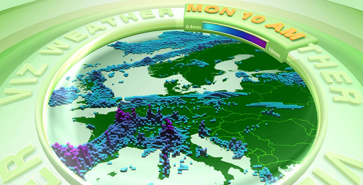
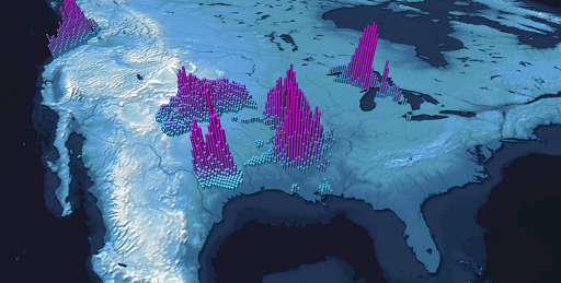
Weather precipitation data
Weather precipitation data clipped to a region
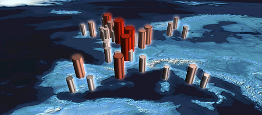
Social TV scene showing population of a particular word in Twitter
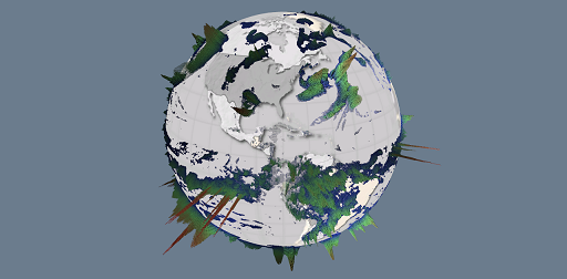
Weather precipitation data on the globe
World temperature values